# Type Analysis via Constant Propagation
## Prelude
While I was working on the C2 compiler in HotSpot, I noticed something
interesting: although Java generics are *erased*, C2 is able to nearly recover
them completely via simple [constant propagation](https://en.wikipedia.org/wiki/Sparse_conditional_constant_propagation).
Afterwards I developed two languages which are directly designed to do all
their type-checking via constant propagation:
[Simple](https://github.com/SeaOfNodes/Simple) and [AA](https://github.com/cliffclick/aa). Both languages are statically typed
and type-safe; AA uses a blend of extended Hindley-Milner and constant propagation.
[Simple](https://github.com/SeaOfNodes/Simple) uses constant propagation
exclusively to do type analysis (and the generate any resulting semantic
errors), and has a working implementation so you can view it in action!
In both languages, after the first round of *pessimistic* constant propagation
(and extensive peephole optimizations) completes, every program point (node in
the IR) has a type - and if there are no error types, then the program is
type-safe. No separate typing pass is needed, and this is typically done
partially as the program parses, finishing shortly thereafter. Optionally, an
*optimistic* constant propagation
([SCCP](https://en.wikipedia.org/wiki/Sparse_conditional_constant_propagation))
can be run to type more programs than the *pessimistic* approach alone.
This discussion relies on the program being in
[SSA](https://en.wikipedia.org/wiki/Static_single-assignment_form)
form, which I assume the reader is familiar with, and is commonly used in
constant propagation because it allows the algorithm to be *sparse* without
effort. Also, all three compilers use the Sea-of-Nodes representation which is
only relevant here because the same SCCP algorithm is now also *conditional* without
any other changes; SCCP does not require the Sea-of-Nodes, although the
presentation is simpler.
More jargon: I use *program points* interchangeably with *nodes in an SSA-based
IR graph* or sometimes simply *nodes*.
## Table of Contents
* [The Basics](#the-basics)
* [More Lattices](#more-lattices)
* [A Sample Typing Error](#a-sample-typing-error)
* [Tuples](#tuples)
* [Structs](#structs)
* [Pointers](#pointers)
* [Functions](#functions)
* [Type Sugar And All The Rest](#type-sugar-and-all-the-rest)
* [Methods](#methods)
* [Subclassing](#Subclassing)
* [Structural Typing](#structural-typing)
* [Nomative Typing and Traits and Interfaces](#nomative-typing-and-traits-and-interfaces)
* [Conditional Conformance](#conditional-conformance)
* [Parametric Polymorphism](#parametric-polymorphism)
* Call Graph Discovery and Separate compilation
* Performance Concerns
* A Self Type
* Overloading
* Typing other simple properties: mutable-or-not, [initialized/destructed]-or-not
* Arrays
## The Basics
Variations of constant propagation have a long history in compilers, and here I
am referring to the well understood
[Monotone Analysis Framework](http://janvitek.org/events/NEU/7580/papers/more-papers/1977-acta-kam-monotone.pdf);
a quick google search finds plethora of courseworks on the topic. I assume the
reader is familiar and I only give a very brief overview here. Constant
propagation has long been used to discover interesting facts about program
points, generally to further optimize a program. We are going to use it to
*type* our programs.
At the core of the problem is a
[lattice](https://en.wikipedia.org/wiki/Lattice_(order)) used to track what values a program point can take on. Here is a common example for tracking integer constants:
[Lattice1](./docs/lattice_i.svg) 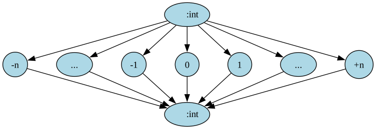 The lattices being used here are:
* Symmetric - every lattice element has a *dual*
* Complete - the *meet* of any two elements is another element
* Bounded (ranked) - the lattice has finite height, which also means there are maximum and minimum elements
and of course the *meet* is idempotent, commutative and associative.
The lattice *join* is defined from the *meet* and *dual* in
the normal way: `~(~x meet ~y)`
Also *isa* is defined as `(x meet y)==y`, e.g. `17.isa(Int)` expands to `(17
meet Int)==Int` which becomes `(Int)==Int` which is `true`.
### The Constant Propagation Algorithm
All nodes are initialized to either *top* ⊤ (SCCP) or *bottom* ⊥ (during
Parsing), and also put on a worklist. We pull work off the worklist until it
runs dry, evaluating the node's *transfer function* to partially evaluate
w.r.t. the lattice. If the evaluation produces a new lattice element, we put
dependent nodes' back on the worklist (using e.g. use-def edges).
```java
while( (node = work.pop()) != null )
if( node.if_changed(node.transfer_fcn()) )
work.addAll( node.uses )
```
The beauty of this algorithm is that it hits a *least fixed point*, a "best
answer" in time proportional to the program size and lattice depth. That
single "best answer" will also become our *typing*, our mapping from program
points' to their *type*.
### Pessmistic vs Optimistic
In general these lattices can be used in either a *pessimistic* or *optimistic*
direction.
The *pessimistic* direction starts with all program points at the least
element, here ⊥, and applies the program points' *transfer function* to
partially evaluate wrt the lattice, potientially discovering new facts or
constants. Another way to think about *bottom* ⊥ is that it represents that
the compiler does not know anything about this value, and that it must emit
code to compute the result the hard way - no shortcuts, no optimizations.
Trivial Example#1:
```python
var x # declare a variable 'x', untyped
x = 2 # assign a 2
print(x) # print x, which is 2
```
Here we see `x=2` at the `print(x)` and this program can be simplified to
`print(2)`, dropping the `x`.
Example#2:
```python
x0 = 1 # Note the SSA renaming
while( rand() ): # Loop an unknown number of times
x1 = φ(x0,x2)
x2 = 2 - x1 # can we discover x2 = 1 here?
print(x1)
```
While evaluating this program from the start, we can see that `x0 = 1` when we
reach the loop entry, but what happens to `x` around the backedge? Since we
start at `⊥` (know nothing), the `φ(x0,x2)` becomes `φ(1,⊥)` which does a
*meet* to yield `⊥` (because the we know nothing about what comes around the
backedge). Then in the loop body `x2 = 2 - x1` becomes `x2 = 2 - ⊥` which is
`⊥` which is what we started with. We have then hit a fixed point with no
values further changing: `x0 = 1; x1 = ⊥; x2 = ⊥`.
Let's repeat Example#2 using the *optimistic* starting point: all values at
`⊤`. An intuition for *top* ⊤ might be "the compiler can pick any convenient
value (as long as the ⊤ is removed before trying to emit code)". Another
intuition might be "top is all possible constants, all at once - an impossible
situation - so later we'll have to pick one (and only one)".
The example is structured a little differently; it interleaves the current
known values for the `x` variables between the lines of code, and follows down
the worklist, and by the loop end shows what we know so-far:
Example#3:
```python
# x0=⊤, x1=⊤, x2=⊤
x0 = 1 # Note the SSA renaming
while( rand() ): # Loop an unknown number of times
# x0=1, x1=⊤, x2=⊤ # x2 is ⊤ around the backedge, instead of ⊥
x1 = φ(x0,x2)
# x0=1, x1=1, x2=⊤
x2 = 2 - x1 # can we discover x2 = 1 here?
# x0=1, x1=1, x2=1
```
Since x2 changed from `⊤` to `1`, we need to repeat uses of x2:
```python
# x0=1, x1=1, x2=1
x1 = φ(x0,x2)
# x0=1, x1=1, x2=1
```
With no change from before and after the `φ(x0,x2)` we hit our fixed point -
and discover that `print(x)` is really `print(1)` and all the `x` math (and the
loop) can be dropped.
The general rule here is that the *optimistic* approach may find more
constants, but never less; while the *pessimistic* approach starts from the
lowest possible types and can be stopped any time yielding a correct analysis
(but a possibly weaker final result). Also the *pessimistic* approach can
be interleaved with other optimizations as long as those optimizations do not lose
any type information - and indeed this is the mode the C2 compiler has been
running in since 1997.
First appears in [Simple chapter02](https://github.com/SeaOfNodes/Simple/tree/main/chapter02):
the pessimistic treatment during parsing with the simple integer lattice.
## More Lattices
We enhance this integer lattice to have a "uber-top" and "uber-bottom",
and rename the existing integer `⊤` and `⊥` to `⊤:int` and `⊥:int`.
We further extend the integers to cover integer ranges; this covers common
language types like `i32`, `i64`, `u16`, `byte`, `bool` and so forth.
[Lattice2](./docs/lattice_i2.svg)
The lattices being used here are:
* Symmetric - every lattice element has a *dual*
* Complete - the *meet* of any two elements is another element
* Bounded (ranked) - the lattice has finite height, which also means there are maximum and minimum elements
and of course the *meet* is idempotent, commutative and associative.
The lattice *join* is defined from the *meet* and *dual* in
the normal way: `~(~x meet ~y)`
Also *isa* is defined as `(x meet y)==y`, e.g. `17.isa(Int)` expands to `(17
meet Int)==Int` which becomes `(Int)==Int` which is `true`.
### The Constant Propagation Algorithm
All nodes are initialized to either *top* ⊤ (SCCP) or *bottom* ⊥ (during
Parsing), and also put on a worklist. We pull work off the worklist until it
runs dry, evaluating the node's *transfer function* to partially evaluate
w.r.t. the lattice. If the evaluation produces a new lattice element, we put
dependent nodes' back on the worklist (using e.g. use-def edges).
```java
while( (node = work.pop()) != null )
if( node.if_changed(node.transfer_fcn()) )
work.addAll( node.uses )
```
The beauty of this algorithm is that it hits a *least fixed point*, a "best
answer" in time proportional to the program size and lattice depth. That
single "best answer" will also become our *typing*, our mapping from program
points' to their *type*.
### Pessmistic vs Optimistic
In general these lattices can be used in either a *pessimistic* or *optimistic*
direction.
The *pessimistic* direction starts with all program points at the least
element, here ⊥, and applies the program points' *transfer function* to
partially evaluate wrt the lattice, potientially discovering new facts or
constants. Another way to think about *bottom* ⊥ is that it represents that
the compiler does not know anything about this value, and that it must emit
code to compute the result the hard way - no shortcuts, no optimizations.
Trivial Example#1:
```python
var x # declare a variable 'x', untyped
x = 2 # assign a 2
print(x) # print x, which is 2
```
Here we see `x=2` at the `print(x)` and this program can be simplified to
`print(2)`, dropping the `x`.
Example#2:
```python
x0 = 1 # Note the SSA renaming
while( rand() ): # Loop an unknown number of times
x1 = φ(x0,x2)
x2 = 2 - x1 # can we discover x2 = 1 here?
print(x1)
```
While evaluating this program from the start, we can see that `x0 = 1` when we
reach the loop entry, but what happens to `x` around the backedge? Since we
start at `⊥` (know nothing), the `φ(x0,x2)` becomes `φ(1,⊥)` which does a
*meet* to yield `⊥` (because the we know nothing about what comes around the
backedge). Then in the loop body `x2 = 2 - x1` becomes `x2 = 2 - ⊥` which is
`⊥` which is what we started with. We have then hit a fixed point with no
values further changing: `x0 = 1; x1 = ⊥; x2 = ⊥`.
Let's repeat Example#2 using the *optimistic* starting point: all values at
`⊤`. An intuition for *top* ⊤ might be "the compiler can pick any convenient
value (as long as the ⊤ is removed before trying to emit code)". Another
intuition might be "top is all possible constants, all at once - an impossible
situation - so later we'll have to pick one (and only one)".
The example is structured a little differently; it interleaves the current
known values for the `x` variables between the lines of code, and follows down
the worklist, and by the loop end shows what we know so-far:
Example#3:
```python
# x0=⊤, x1=⊤, x2=⊤
x0 = 1 # Note the SSA renaming
while( rand() ): # Loop an unknown number of times
# x0=1, x1=⊤, x2=⊤ # x2 is ⊤ around the backedge, instead of ⊥
x1 = φ(x0,x2)
# x0=1, x1=1, x2=⊤
x2 = 2 - x1 # can we discover x2 = 1 here?
# x0=1, x1=1, x2=1
```
Since x2 changed from `⊤` to `1`, we need to repeat uses of x2:
```python
# x0=1, x1=1, x2=1
x1 = φ(x0,x2)
# x0=1, x1=1, x2=1
```
With no change from before and after the `φ(x0,x2)` we hit our fixed point -
and discover that `print(x)` is really `print(1)` and all the `x` math (and the
loop) can be dropped.
The general rule here is that the *optimistic* approach may find more
constants, but never less; while the *pessimistic* approach starts from the
lowest possible types and can be stopped any time yielding a correct analysis
(but a possibly weaker final result). Also the *pessimistic* approach can
be interleaved with other optimizations as long as those optimizations do not lose
any type information - and indeed this is the mode the C2 compiler has been
running in since 1997.
First appears in [Simple chapter02](https://github.com/SeaOfNodes/Simple/tree/main/chapter02):
the pessimistic treatment during parsing with the simple integer lattice.
## More Lattices
We enhance this integer lattice to have a "uber-top" and "uber-bottom",
and rename the existing integer `⊤` and `⊥` to `⊤:int` and `⊥:int`.
We further extend the integers to cover integer ranges; this covers common
language types like `i32`, `i64`, `u16`, `byte`, `bool` and so forth.
[Lattice2](./docs/lattice_i2.svg) 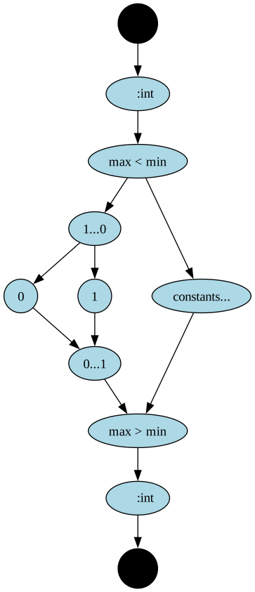 First appears in [Simple chapter14](https://github.com/SeaOfNodes/Simple/tree/main/chapter14).
Parallel to the integer lattice we add a IEEE 754 floating point lattice, which
allows us to track FP constants, e.g. `0.` or `pi`. We track both 32b and 64b
values, and can observe that the 32b ones are a strict subset of the 64b ones.
[Lattice3](./docs/lattice_if.svg)
First appears in [Simple chapter14](https://github.com/SeaOfNodes/Simple/tree/main/chapter14).
Parallel to the integer lattice we add a IEEE 754 floating point lattice, which
allows us to track FP constants, e.g. `0.` or `pi`. We track both 32b and 64b
values, and can observe that the 32b ones are a strict subset of the 64b ones.
[Lattice3](./docs/lattice_if.svg) 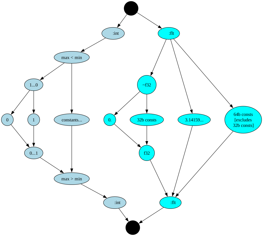 First appears in [Simple chapter12](https://github.com/SeaOfNodes/Simple/tree/main/chapter12).
Now we add more "inner" lattices, the key being that inner lattices do not
themselves contain another lattice element. For example a hypothetical
sub-word FP format:
[Lattice4](./docs/lattice_iff.svg)
First appears in [Simple chapter12](https://github.com/SeaOfNodes/Simple/tree/main/chapter12).
Now we add more "inner" lattices, the key being that inner lattices do not
themselves contain another lattice element. For example a hypothetical
sub-word FP format:
[Lattice4](./docs/lattice_iff.svg) 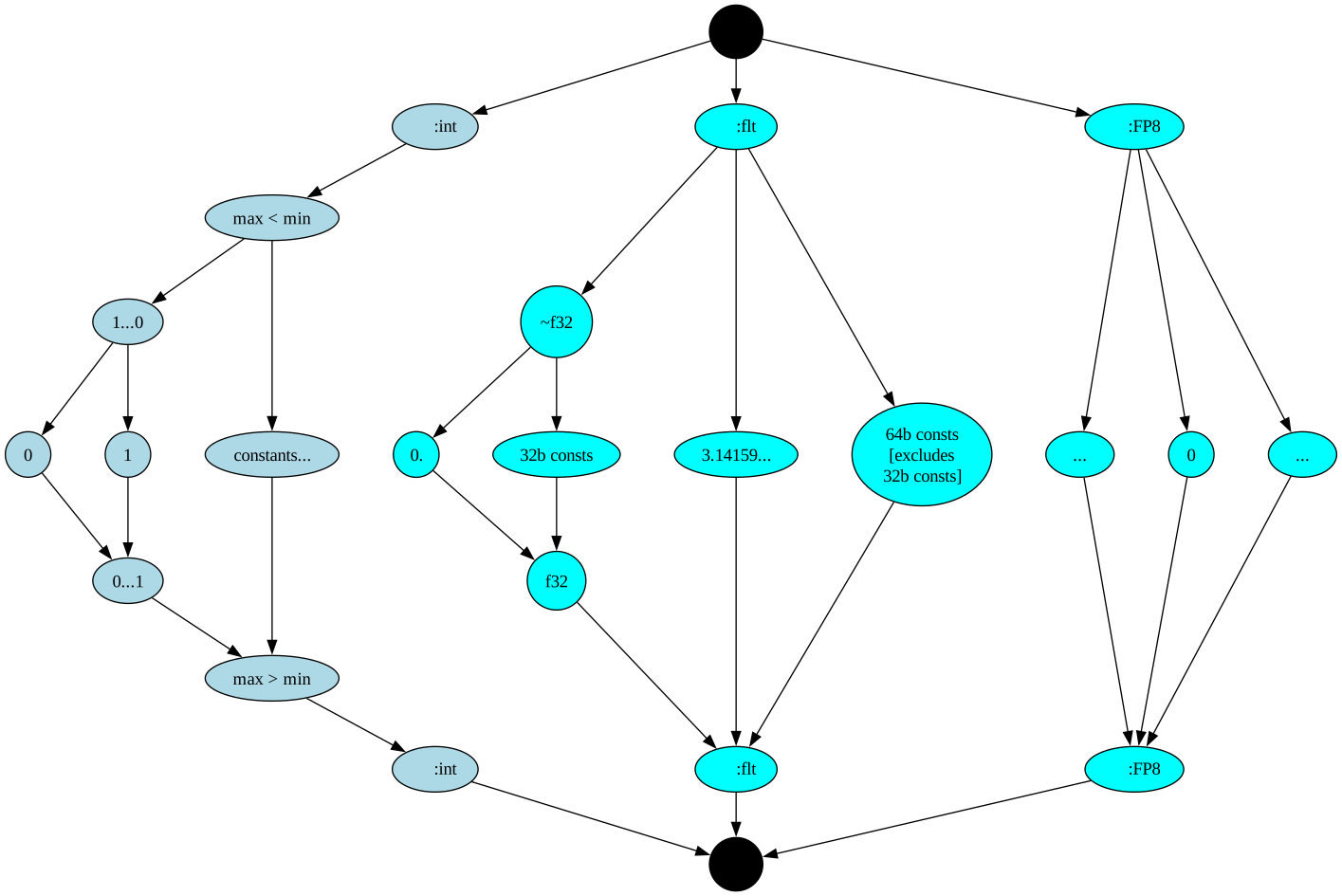 A *control* type, used to signify that a Node is reachable or dead. These
show up in the *conditional* part of SCCP when analyzing e.g.
```python
test = False;
if test:
dead_code
```
[Lattice5](./docs/lattice_iffc.svg)
A *control* type, used to signify that a Node is reachable or dead. These
show up in the *conditional* part of SCCP when analyzing e.g.
```python
test = False;
if test:
dead_code
```
[Lattice5](./docs/lattice_iffc.svg) 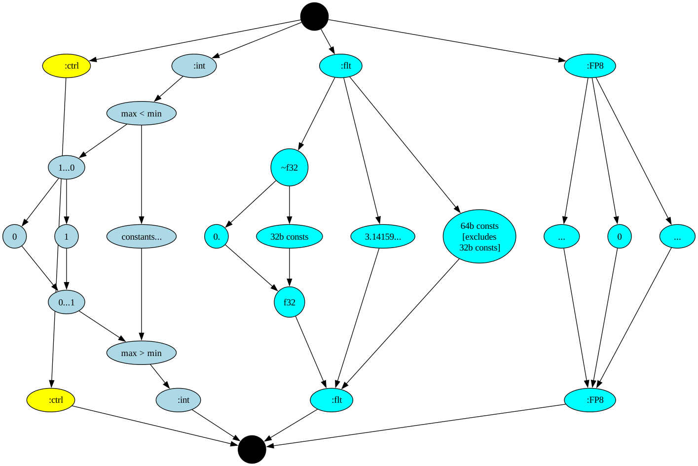 First appears in [Simple chapter04](https://github.com/SeaOfNodes/Simple/tree/main/chapter04).
Hopefully it is clear how to add another sub-lattice that itself is symmetric,
complete and ranked.
## A Sample Typing Error
```python
var x = 1
x = 3.14
```
Here `x` is given a type, which the language parser records with the expression
defining `x`. i.e., `x` is currently typed as a `1` (also has the *value* `1`,
which is not the same thing). Generally this is too restrictive a type to be
desirable, so commonly the parser widens the type `1` to e.g. `int64` or `Int`.
After the initial type inference for `x`, further updates are guarded by a
*type cast*, an IR Node which *meets* any assigned value with the inferred type
for `x`. If the *meet* hits `⊥`, this signifies a type error.
This is in general how we handle type errors: at user added type ascriptions,
declarations on structs or classes, or any place a type is known, we insert a
*type cast* in the IR. The *type cast* should eventually become redundant and
fold away. If the incoming type *isa* the internal type, the cast is a no-op.
If it does not, it is a type error.
## Tuples
So far our lattice is composed of a series of sub-lattices joined by an
"uber-top" and "uber-bottom", and each sub-lattice in turn is composed of
various type base elements (e.g. 'int' or '3.14').
Now we introduce a collection of lattice elements, as itself a lattice.
Examples might be `[Ctrl, 17]` or `[3.14, ⊤:int, 0:FP8]`, or `[3.14, 17,
⊥:FP8]`.
*Meet* on these tuples is defined element wise; looking at the last two examples
the meet is `[3.14 meet 3.14, ⊤:int meet 17, 0:FP8 meet ⊥:FP8]` which folds to
`[3.14, 17, ⊥:FP8]`.
We also need to handle when the number of elements does not match, such as
`[Ctrl, 17]` meet `[3.14, 17, ⊥:FP8]`. Meeting such mismatches is required to
keep our lattice *complete*. In general there are two obvious ways forward:
fall hard to ⊥, or try to preserve some knowledge. Falling hard to ⊥ basically
declares a type error and is probably correct in some situations. However
preserving knowledge is really helpful during type inference and is absolutely
required in a few cases, so we use the other plan: every tuple has some prefix
of interesting values, and an infinite number of trailing ⊥ (or ⊤) fields, not
printed for brevity.
`[Ctrl, 17]` is really: `[Ctrl, 17, ⊥, ⊥, ⊥, ....]`.
`[3.14, 17, ⊥:FP8]` is really `[3.14, 17, ⊥:FP8, ⊥, ⊥, ⊥, ....]`.
Their meet is then:
`[⊥, 17, ⊥, ⊥, ⊥, ....]` (which prints as: `[⊥, 17]`)
and our lattice is once again complete.
Tuples by themselves are not terribly interesting (or common in programming)
but we will shortly use them in building structs and functions.
[Lattice6](./docs/lattice_iffct.svg)
First appears in [Simple chapter04](https://github.com/SeaOfNodes/Simple/tree/main/chapter04).
Hopefully it is clear how to add another sub-lattice that itself is symmetric,
complete and ranked.
## A Sample Typing Error
```python
var x = 1
x = 3.14
```
Here `x` is given a type, which the language parser records with the expression
defining `x`. i.e., `x` is currently typed as a `1` (also has the *value* `1`,
which is not the same thing). Generally this is too restrictive a type to be
desirable, so commonly the parser widens the type `1` to e.g. `int64` or `Int`.
After the initial type inference for `x`, further updates are guarded by a
*type cast*, an IR Node which *meets* any assigned value with the inferred type
for `x`. If the *meet* hits `⊥`, this signifies a type error.
This is in general how we handle type errors: at user added type ascriptions,
declarations on structs or classes, or any place a type is known, we insert a
*type cast* in the IR. The *type cast* should eventually become redundant and
fold away. If the incoming type *isa* the internal type, the cast is a no-op.
If it does not, it is a type error.
## Tuples
So far our lattice is composed of a series of sub-lattices joined by an
"uber-top" and "uber-bottom", and each sub-lattice in turn is composed of
various type base elements (e.g. 'int' or '3.14').
Now we introduce a collection of lattice elements, as itself a lattice.
Examples might be `[Ctrl, 17]` or `[3.14, ⊤:int, 0:FP8]`, or `[3.14, 17,
⊥:FP8]`.
*Meet* on these tuples is defined element wise; looking at the last two examples
the meet is `[3.14 meet 3.14, ⊤:int meet 17, 0:FP8 meet ⊥:FP8]` which folds to
`[3.14, 17, ⊥:FP8]`.
We also need to handle when the number of elements does not match, such as
`[Ctrl, 17]` meet `[3.14, 17, ⊥:FP8]`. Meeting such mismatches is required to
keep our lattice *complete*. In general there are two obvious ways forward:
fall hard to ⊥, or try to preserve some knowledge. Falling hard to ⊥ basically
declares a type error and is probably correct in some situations. However
preserving knowledge is really helpful during type inference and is absolutely
required in a few cases, so we use the other plan: every tuple has some prefix
of interesting values, and an infinite number of trailing ⊥ (or ⊤) fields, not
printed for brevity.
`[Ctrl, 17]` is really: `[Ctrl, 17, ⊥, ⊥, ⊥, ....]`.
`[3.14, 17, ⊥:FP8]` is really `[3.14, 17, ⊥:FP8, ⊥, ⊥, ⊥, ....]`.
Their meet is then:
`[⊥, 17, ⊥, ⊥, ⊥, ....]` (which prints as: `[⊥, 17]`)
and our lattice is once again complete.
Tuples by themselves are not terribly interesting (or common in programming)
but we will shortly use them in building structs and functions.
[Lattice6](./docs/lattice_iffct.svg) 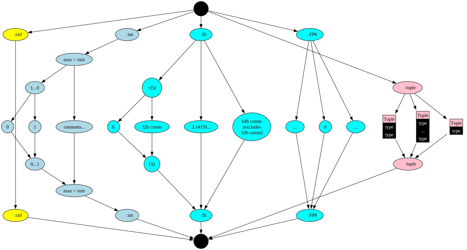 First appears in [Simple chapter10a](https://github.com/SeaOfNodes/Simple/tree/main/chapter10a)
along with structs and pointers.
## Structs
We implement *struct types* as a tuple with named fields:
`[myPi: 3.14, result: 17, someFP8: ⊥:FP8]`
The field ordering is not important (and indeed in many languages the compiler
is free to re-order fields to achieve a better packing density). For the
trailing infinitely many ⊥ fields, we can find all possible field names in the
infinite set.
Actually, to cut down the number of cases we need to handle, we define tuples
as *structs* with numbers for field names: `[0,1,2,3...]`
The actual implementation of structs might use hash tables to map unordered
field strings to types, or might use linear scan for small structs.
[Lattice7](./docs/lattice_iffcs.svg)
First appears in [Simple chapter10a](https://github.com/SeaOfNodes/Simple/tree/main/chapter10a)
along with structs and pointers.
## Structs
We implement *struct types* as a tuple with named fields:
`[myPi: 3.14, result: 17, someFP8: ⊥:FP8]`
The field ordering is not important (and indeed in many languages the compiler
is free to re-order fields to achieve a better packing density). For the
trailing infinitely many ⊥ fields, we can find all possible field names in the
infinite set.
Actually, to cut down the number of cases we need to handle, we define tuples
as *structs* with numbers for field names: `[0,1,2,3...]`
The actual implementation of structs might use hash tables to map unordered
field strings to types, or might use linear scan for small structs.
[Lattice7](./docs/lattice_iffcs.svg) 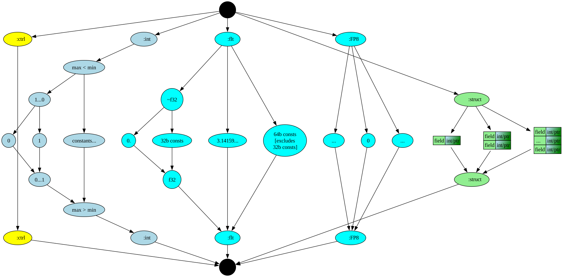 Struct fields can have more properties than a name; easy examples include
`initialized` or not, `mutable` or not, `destructed` not. Adding some boolean
properties here does not fundamentally change how a field works; the field
*meet* operations will either AND or OR these properties according to the
desired semantics, as well as the normal *meet* on the field type.
I am not covering here how to initialize struct members, or the syntax for
declaring structs or traits - just the resulting types.
First appears in [Simple chapter10a](https://github.com/SeaOfNodes/Simple/tree/main/chapter10a)
along with tuples and pointers.
## Pointers
We implement typed pointers as a wrapper over a struct, with extra bits
for carrying more information depending on the level of precision desired.
[Lattice8](./docs/lattice_iffcsp.svg)
Struct fields can have more properties than a name; easy examples include
`initialized` or not, `mutable` or not, `destructed` not. Adding some boolean
properties here does not fundamentally change how a field works; the field
*meet* operations will either AND or OR these properties according to the
desired semantics, as well as the normal *meet* on the field type.
I am not covering here how to initialize struct members, or the syntax for
declaring structs or traits - just the resulting types.
First appears in [Simple chapter10a](https://github.com/SeaOfNodes/Simple/tree/main/chapter10a)
along with tuples and pointers.
## Pointers
We implement typed pointers as a wrapper over a struct, with extra bits
for carrying more information depending on the level of precision desired.
[Lattice8](./docs/lattice_iffcsp.svg) 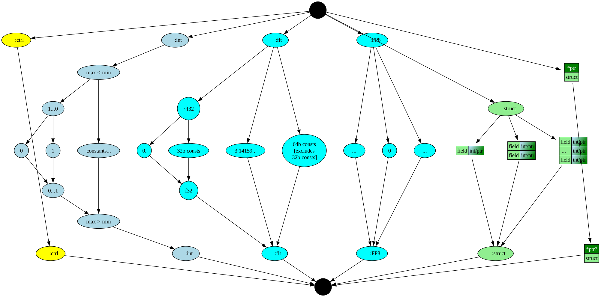 Tracking null pointers is easy this way, with a simple lattice `{ ⊤, ptr, ptr?, ⊥}` where the `ptr?`
indicates a pointer which may be null. We can make dereferencing a may-be-null pointer
safe with a runtime check and an upcast:
```
// Inferred type: *?[name:"Whiskers", makeSound:#1{}]
// Pronounced: pointer-to-a-nullable-Cat
val ptr = rand() ? null : Cat("Whiskers");
// null-check
if( ptr )
// hidden upcast to drop the null
ptr.makeSound() // Legal, because ptr cannot be null
```
The same code with a "possibly null pointer" error:
```
// Same as above:
// Inferred type: *?[name:"Whiskers", makeSound:#1{}]
// Pronounced: pointer-to-a-nullable-Cat
val ptr = rand() ? null : Cat("Whiskers");
// Illegal, because ptr might be null
ptr.makeSound() // TYPE ERROR!
```
Here the load to fetch the `makeSound` method fails during error reporting; in
Simple this is just a `LoadNode` which has an error check against its pointer
input being possibly `null`.
First appears in [Simple chapter10a](https://github.com/SeaOfNodes/Simple/tree/main/chapter10a),
along with structs and tuples.
### Equivalence Class Aliasing
The Sea-of-Nodes IR design uses the *equivalence class* model of aliasing,
where memory is broken up into *equivalence classes*. Pointers point into one
or another class; pointers in unrelated classes **never** alias, those in the
same class **always** alias.
This model works really well for strongly typed languages such as Java and
Simple. I believe it will work well for other strongly typed languages as
well, although I have not tried it. Obviously other models work as well. In
this case it is easy to add aliasing support in the type system: all fields
have an *alias number*, a unique indicator of which *equivalence class* they
belong too. Set of aliases are possible, often implemented with a bitvector.
In the above example with a struct `[myPi: 3.14, result: 17, someFP8: ⊥:FP8]`
memory is broken up into classes for the `myPi` fields, `result` fields and
`someFP8` fields, leading to at least 3 alias classes. Pointers to the `myPi`
fields will never alias with `result` fields because the field names are
different (also, the core types are different).
Pointer types may also carry information like `raw` or `unsafe`, or pointers
into e.g. GPU memory (probably as another alias class), or pointers to
uninitialized memory, or destructed memory or singletons.
## Functions
Functions have argument types and some return types (often just one return
type). We'll model them as an argument struct and a return struct (or type if
the language only allows 1 return).
Because of co-variance/contra-variance, the two structs are treated slightly
differently: the arguments will *joined* and the returns will be *meet*.
Example:
```java
var fcn = rand()
? fcn_widen_ascii_char:{u8 -> u16}
: fcn_narrow_wide_char:{u16 -> u8};
var some_ary = map(get_u8_ary(), fcn);
```
What is the type of the `fcn` variable? It is a function which takes either a
`u8` or `u16`... which means the best `map` can hope for is that `fcn` can only
be passed `u8`s, and not something in the `u16` range. Similarly for the
result, `map` might see `u16`s if `fcn_widen_ascii_char` is being called.
`fcn`'s type is the meet of `fcn_widen_ascii_char` and `fcn_narrow_wide_char`
which is
`fcn: {u8 -> u16}.meet( {u16 -> u8 } )`
`fcn: { u8.join(u16) -> u16.meet(u8) }`
`fcn: { u8 -> u16 }`
### Function Indices
There are a finite number of functions in any fixed program; it is useful to
name them (even if anonymous!) so the type system can reason about them.
The type for `fcn` might also include the functions it is built from,
so e.g. `fcn: [fcn_widen_ascii_char,fcn_narrow_wide_char]{u8 -> u16}`.
Collections of possible functions are easy to track as e.g. a simple bitvector,
with one bit for each function in the program. Other choices also work, such
as a sparse bitvector when only a few functions are possible from a large
program with many 1000's of functions. The most common function type is that
of a single function, i.e., just calling a function by name.
A *function index* is simply a unique small integer that refers to a function
(perhaps via array lookup), and can be efficiently tracked. We print them as
`[#fidxs]{signature -> return}` The above `fcn` is typed `[#2,3]{u8 -> u16}`,
indicating both function #2 and function #3 are included here.
The type system will track function collections *in general*, so the general
case is that the function type has a set of allowed functions, and might
include an indication of the infinite number of functions that might be found
in some external compilation unit.
The reason to track functions this way is that the type system will allow us to
build a reasonably accurate Call Graph: the set of function types arriving at a call
site dictates which functions might be called here. More on this in the [Call
Graph](#call-graph) section.
First appears in [Simple chapter18](https://github.com/SeaOfNodes/Simple/tree/main/chapter18).
## Type Sugar And All The Rest
From here on out, we will mostly be adding a small amount of *type sugar*
to the existing types to implement all the cool type features we want.
Methods, SubClassing, Structural-Typing, and Traits will all be handled via *type
sugar*. I *believe* (not directly implemented as of today), Conditional
Conformances will fall out as a case of structural-typing, which *is* handled here.
## Methods
In many languages, structs have *methods*, functions which take a `self` or
`this` extra argument from the struct itself.
```java
struct String {
String toUpperCase(/*hidden this argument */) { ... };
}
```
In this typing formulation, methods will be **fields** that happen to be
function-typed, or basically as type sugar over the existing types already
mentioned above.
The `toUpperCase` field here is **finally** assigned a function constant - and,
as with all final constant fields, the field value is the same for all
instances of `String` so does not need to be implemented as actually in the
`String` instances. As an implementation detail, these final field constants
can be moved over to some collection of such constant fields, e.g. a `class String`
instance.
From the typing systems point-of-view, the field is a full-fledged
member of the `String` type. E.g. some pseudo-definition of `String`:
```java
String = : { // String is a struct type...
toUpperCase // with a field called toUpperCase...
: [#1]{ String -> String }, // typed as a function from String to String
... // And probably has many more fields, elided here
};
```
Here is a method call `"abc".toUpperCase()` from the type systems'
point-of-view: There is a field lookup `toUpperCase`, which needs to be found
in the struct type for `"abc"`; that needs to return a no-arg (plus `self`)
function which will be called.
```
Code Type
"abc" : {toUpperCase:[#1]{String->String}, ...other fields}
.toUpperCase : [#1]{String->String} // Just the field contents, which is a function
("abc") String // Call fcn#1 with self
```
When is a special String type e.g. UTF8String *isa* String? Exactly when the *isa* call
returns `True`; when UTF8String has all the same fields as a `String` (and
probably has more).
This is the general way *methods* are handled: they are reduced to function-
typed fields in a struct, and then the existing *meet* and *join* operations
are well defined.
First appears in [Simple chapter23](https://github.com/SeaOfNodes/Simple/tree/main/chapter23).
## Subclassing
As alluded to in the prior section, sub-classing is a modest amount of *type
sugar* over the existing struct types. Here is a generic example with totally
made-up syntax:
```java
// An abstract Pet class
Pet = : {
name: String
makeSound: { Self -> String } = 0;// function pointer is null; this class is *abstract*
};
// Cat is a sub-class of Pet, and concretely defines `makeSound`
Cat = : Pet : {
makeSound = { self -> "meow" };
};
cat = Cat("Whiskers");
// Another sub-class of Pet
Dog = : Pet : {
makeSound = { self -> "bark" };
};
dog = Dog("Spot");
```
`Pet` is a name for a type `[name:String, makeSound:[#0]{Pet->String}]`. The
`makeSound` field is typed with a null function pointer, shown as `[#0]`.
`Cat` is a name for a type `[name:String, makeSound:[#1]{Pet->String}]`,
i.e. it is a `Pet` except the `makeSound` field is now typed as a concrete
function `[#1]`. Similarly, for `Dog` and concrete function `[#2]`
The instance variable `cat` is typed as `[name:"Whiskers",
makeSound:[#1]{Pet->String}]` which *isa* `Cat`, and similar for `dog` and
`Dog`.
`cat.isa(Cat)` and `Cat.isa(Pet)` and
`dog.isa(Dog)` and `Dog.isa(Pet)`.
Subclassing generally means supporting *virtual* calls, so here I will show a
typical virtual call execution strategy; other strategies are possible
(e.g. *inline caches* in some VMs). In this case, the optimized version of
methods means moving from the instance to the class, then doing the field
lookup to get a function... then calling it. This is the same sequence as done
by both C++ and Java.
`(rand() ? cat : dog).makeSound()`
An implementation in psuedo-asm:
```
rPet = ... # pick one of cat or dog
rClass = ld.ptr (rPet+#classOffset)
rSound = ld.ptr (rClass+#fieldOffsetMakeSound)
call (rSound)
```
Another issue is handling shadowing of fields; when a subclass adds a new field
with the same name as a prior one. The parser will need a "shadow-smart"
lookup mechanism, not discussed here. From the type systems point-of-view, we
would like to define a subclass as simply the normal (super-class) struct with
some extra fields. We can use name mangling to keep the fields apart as one
simple solution; there are other solutions such as stacked successive lookups
when checking on fields.
## Structural Typing
We already have structural typing (e.g. static duck-typing) with no further
ado. Here we make a struct type with a single field `quack`, and an infinite
number of `⊤` fields, meaning we don't care what the other fields are. This
type is more-or-less an *interface* or *trait* without a name.
```
{quack : { self -> String }, ⊤, ⊤, ⊤,,, }
```
The `quackathon` function checks that the caller passes in a struct with the
`quack` field:
```
quackathon = { arg: {quack : { self -> String }, ⊤, ⊤, ⊤,,, } ->
arg.quack();
}
```
Any argument type that matches that signature is allowed; the *type cast* used
to check the types just does a *meet* with the incoming argument; if the
incoming argument lacks a `quack` field, it will take the default `⊥` from the
argument, and will lack a `quack` field... which will type error at the field load.
```
Duck : Pet : {
makeSound = { self -> "quack" }
quack = makeSound();
};
StealthCow : Pet : {
makeSound = { self -> "moo" }
quack = { self -> "quack" }
};
```
Both of these types have a `quack` function-typed field, so both are legal
here. The requirement is strictly that the passed-in argument has the needed
signature (needs a function-typed `quack` field).
However if we try to call `dog.quack()`, we will attempt to lookup the `quack`
field in the `Dog` type. `Dog` does not explicity have such a field, and so we
get the default field type: `quack:⊥` which we then try to treat as a
function... and since `⊥` is not a function type we get a type error.
## Nominative Typing and Traits and Interfaces
Nominative typing is basically structural typing, plus a constraint that we
*also* match the type name. If you do not structurally type, you'll also fail
nominative typing, but not vice-versa. We add a little type sugar to force a
failure if the type names do not match, a hidden field with a funny name:
```java
Duck : Pet : {
$classDuck : 0; // hidden field with mangled class name
makeSound = { self -> "quack" }
quack = makeSound();
};
StealthCow : Pet : {
$classStealthCow : 0; // hidden field with mangled class name
makeSound = { self -> "moo" }
quack = { self -> "quack" }
};
```
And now we need to constrain our `quackathon` to only allow `Duck`s:
```
quackathon = { arg: Duck ->
*type cast check Duck*
arg.quack();
}
```
### Nominative Typing Error Example
This code works as expected (Donald enters the quackathon):
`quackathon(Duck("Donald"))`
and this fails:
`quackathon(StealthCow("Betsy"))`
because although `StealthCow` quacks like a duck, it does not have the required
`$classDuck` field; this field goes to `⊥` and the *type cast* will fail.
Let's expand on this fail to make it more explicit:
There is a *type cast* that the arguments are correct; it does a *isa* check
with the input and expected type, and if the the argument is not *isa*, will
flag a type error at the time of *type analysis* (i.e. constant propagation).
Unlike *structural typing*, where we require a `quack` field from the argument
via directly loading a `quack` field, here we require the `$classDuck` field.
The argument type to the second `quackathon` call is a `StealthCow` which
expands to:
```java
{
$classPet: 0; // StealthCow is also a Pet
$classDuck: ⊥; // All other fields are ⊥
$classStealthCow: 0;
name: "Betsy"; // StealthCows are Pets, which have a name
makeSound = #3{ self -> "moo" }; // function index #3
quack = #4{ self -> "quack" };
// all other fields are ⊥
...
}
```
The check is against a generic `Duck` which expands to:
```java
{
$classPet: 0; // Duck is also a Pet
$classDuck: 0; //
$classStealthCow: ⊥; // All other fields are ⊥
name: String; // Ducks are Pets which have a name
makeSound = #5{ self -> "quack" }; // function index #3
quack = #5{ self -> "quack" };
// all other fields are ⊥
...
}
```
The *isa* check is `(StealthCow meet Duck) == Duck`. The *meet* of
StealthCow and Duck is done field by field and results in:
```java
{
$classPet: 0; // Since both are Pets, this field remains
$classDuck: ⊥; // Not really a Duck, the meet lacks $classDuck
$classStealthCow: ⊥; // Not really a StealthCow, the meet lacks $classStealthCow
name: String; // Generic name from the generic Pet
makeSound = #[3,5]{ Pet -> String }; // function indices #3,5
quack = #[4,5]{ Pet -> "quack" }; // function indices #4,5
}
```
And since this is not equal to a `Duck` (the `$classDuck` field is
missing/default and not `0`) , the `isa` returns false, the *type cast* will
report an error.
### A Trait Example
Let's make a concrete working example with a trait `Equals`; here is the
type for `Equals`:
```java
Equals = : { // Equals is a struct (trait) with...
eq = { Self Self -> bool }; // With a field 'eq' typed as a function taking 2 selfs
⊤, ⊤, ⊤,,, // And the infinite unknown fields are ⊤ ... allowing anything
};
```
From the above example with `Duck`s and `Cow`s, we can see they are not `Equals` (will fail
the *isa* test) because they lack an `eq` function. No two Ducks are the same.
Lets make our `String`s equatable:
```java
String = : {
eq = { String String -> bool };
... // plus all the other String stuff
};
```
And Strings can be compared with in code which declares String:
```java
isHappy = { str : String -> str.eq("Happy") }
```
Although code using Pets fails here:
```java
isHappy = { pet : Pet -> pet.eq("Happy") }
ERROR: No field `eq` on type Pet
```
And if we reverse the calling arguments:
```java
isHappy = { pet : Pet -> "Happy".eq(pet) }
ERROR: function String.eq argument#1 must be a String and not a Pet
```
## Parametric Polymorphism
**TODO**...
This looks to me to be solved with **specialization** (cloning the analysis in
any work should work, function inlining or function specialization are both
ways to clone the analysis).
Type var with the intent it becomes concrete - treat as bot/top, maybe not
even need specialized name ?
Trigger inline/specialize based on having concrete args to a function w/ type
var (Parm with a default BOT type). After specialize, Parm with lift to the
concrete and problem solved...
Specialization will split FIDXs, will need to deal with that (keep precise
Call Graph)
## Conditional Conformance
"Conditional Conformance" is a fancy name for a fairly simple idea: if an
Element has a property, then a Collection of such Elements also has that
property, and if not then not. An example might be something that is
`Stringable`, then a collection of them is also `Stringable`, perhaps as
printing as `[elem0,elem1,...]`. Same for e.g. `Equatable` or `Hashable` or `Comparable`.
The Collection defines how to extend the base notion. So e.g. a collection of
`Comparable`s is itself comparable, and that comparison might either return an
element-wise collection of `Bool`s, or might compare lexigraphically and return a
single `Bool` instead of a collection.
However, the collection can also work with elements that are not `Comparable`,
in which case the entire collection is not `Comparable`... but it still
functions as a collection.
So, conditional on the element having a trait `T`, the entire collection also has trait `T`.
So how does that work here?
**TODO**...
Expand to remove polymorphism (above)
Structual typing gives the answer.
Can refine further.
Tracking null pointers is easy this way, with a simple lattice `{ ⊤, ptr, ptr?, ⊥}` where the `ptr?`
indicates a pointer which may be null. We can make dereferencing a may-be-null pointer
safe with a runtime check and an upcast:
```
// Inferred type: *?[name:"Whiskers", makeSound:#1{}]
// Pronounced: pointer-to-a-nullable-Cat
val ptr = rand() ? null : Cat("Whiskers");
// null-check
if( ptr )
// hidden upcast to drop the null
ptr.makeSound() // Legal, because ptr cannot be null
```
The same code with a "possibly null pointer" error:
```
// Same as above:
// Inferred type: *?[name:"Whiskers", makeSound:#1{}]
// Pronounced: pointer-to-a-nullable-Cat
val ptr = rand() ? null : Cat("Whiskers");
// Illegal, because ptr might be null
ptr.makeSound() // TYPE ERROR!
```
Here the load to fetch the `makeSound` method fails during error reporting; in
Simple this is just a `LoadNode` which has an error check against its pointer
input being possibly `null`.
First appears in [Simple chapter10a](https://github.com/SeaOfNodes/Simple/tree/main/chapter10a),
along with structs and tuples.
### Equivalence Class Aliasing
The Sea-of-Nodes IR design uses the *equivalence class* model of aliasing,
where memory is broken up into *equivalence classes*. Pointers point into one
or another class; pointers in unrelated classes **never** alias, those in the
same class **always** alias.
This model works really well for strongly typed languages such as Java and
Simple. I believe it will work well for other strongly typed languages as
well, although I have not tried it. Obviously other models work as well. In
this case it is easy to add aliasing support in the type system: all fields
have an *alias number*, a unique indicator of which *equivalence class* they
belong too. Set of aliases are possible, often implemented with a bitvector.
In the above example with a struct `[myPi: 3.14, result: 17, someFP8: ⊥:FP8]`
memory is broken up into classes for the `myPi` fields, `result` fields and
`someFP8` fields, leading to at least 3 alias classes. Pointers to the `myPi`
fields will never alias with `result` fields because the field names are
different (also, the core types are different).
Pointer types may also carry information like `raw` or `unsafe`, or pointers
into e.g. GPU memory (probably as another alias class), or pointers to
uninitialized memory, or destructed memory or singletons.
## Functions
Functions have argument types and some return types (often just one return
type). We'll model them as an argument struct and a return struct (or type if
the language only allows 1 return).
Because of co-variance/contra-variance, the two structs are treated slightly
differently: the arguments will *joined* and the returns will be *meet*.
Example:
```java
var fcn = rand()
? fcn_widen_ascii_char:{u8 -> u16}
: fcn_narrow_wide_char:{u16 -> u8};
var some_ary = map(get_u8_ary(), fcn);
```
What is the type of the `fcn` variable? It is a function which takes either a
`u8` or `u16`... which means the best `map` can hope for is that `fcn` can only
be passed `u8`s, and not something in the `u16` range. Similarly for the
result, `map` might see `u16`s if `fcn_widen_ascii_char` is being called.
`fcn`'s type is the meet of `fcn_widen_ascii_char` and `fcn_narrow_wide_char`
which is
`fcn: {u8 -> u16}.meet( {u16 -> u8 } )`
`fcn: { u8.join(u16) -> u16.meet(u8) }`
`fcn: { u8 -> u16 }`
### Function Indices
There are a finite number of functions in any fixed program; it is useful to
name them (even if anonymous!) so the type system can reason about them.
The type for `fcn` might also include the functions it is built from,
so e.g. `fcn: [fcn_widen_ascii_char,fcn_narrow_wide_char]{u8 -> u16}`.
Collections of possible functions are easy to track as e.g. a simple bitvector,
with one bit for each function in the program. Other choices also work, such
as a sparse bitvector when only a few functions are possible from a large
program with many 1000's of functions. The most common function type is that
of a single function, i.e., just calling a function by name.
A *function index* is simply a unique small integer that refers to a function
(perhaps via array lookup), and can be efficiently tracked. We print them as
`[#fidxs]{signature -> return}` The above `fcn` is typed `[#2,3]{u8 -> u16}`,
indicating both function #2 and function #3 are included here.
The type system will track function collections *in general*, so the general
case is that the function type has a set of allowed functions, and might
include an indication of the infinite number of functions that might be found
in some external compilation unit.
The reason to track functions this way is that the type system will allow us to
build a reasonably accurate Call Graph: the set of function types arriving at a call
site dictates which functions might be called here. More on this in the [Call
Graph](#call-graph) section.
First appears in [Simple chapter18](https://github.com/SeaOfNodes/Simple/tree/main/chapter18).
## Type Sugar And All The Rest
From here on out, we will mostly be adding a small amount of *type sugar*
to the existing types to implement all the cool type features we want.
Methods, SubClassing, Structural-Typing, and Traits will all be handled via *type
sugar*. I *believe* (not directly implemented as of today), Conditional
Conformances will fall out as a case of structural-typing, which *is* handled here.
## Methods
In many languages, structs have *methods*, functions which take a `self` or
`this` extra argument from the struct itself.
```java
struct String {
String toUpperCase(/*hidden this argument */) { ... };
}
```
In this typing formulation, methods will be **fields** that happen to be
function-typed, or basically as type sugar over the existing types already
mentioned above.
The `toUpperCase` field here is **finally** assigned a function constant - and,
as with all final constant fields, the field value is the same for all
instances of `String` so does not need to be implemented as actually in the
`String` instances. As an implementation detail, these final field constants
can be moved over to some collection of such constant fields, e.g. a `class String`
instance.
From the typing systems point-of-view, the field is a full-fledged
member of the `String` type. E.g. some pseudo-definition of `String`:
```java
String = : { // String is a struct type...
toUpperCase // with a field called toUpperCase...
: [#1]{ String -> String }, // typed as a function from String to String
... // And probably has many more fields, elided here
};
```
Here is a method call `"abc".toUpperCase()` from the type systems'
point-of-view: There is a field lookup `toUpperCase`, which needs to be found
in the struct type for `"abc"`; that needs to return a no-arg (plus `self`)
function which will be called.
```
Code Type
"abc" : {toUpperCase:[#1]{String->String}, ...other fields}
.toUpperCase : [#1]{String->String} // Just the field contents, which is a function
("abc") String // Call fcn#1 with self
```
When is a special String type e.g. UTF8String *isa* String? Exactly when the *isa* call
returns `True`; when UTF8String has all the same fields as a `String` (and
probably has more).
This is the general way *methods* are handled: they are reduced to function-
typed fields in a struct, and then the existing *meet* and *join* operations
are well defined.
First appears in [Simple chapter23](https://github.com/SeaOfNodes/Simple/tree/main/chapter23).
## Subclassing
As alluded to in the prior section, sub-classing is a modest amount of *type
sugar* over the existing struct types. Here is a generic example with totally
made-up syntax:
```java
// An abstract Pet class
Pet = : {
name: String
makeSound: { Self -> String } = 0;// function pointer is null; this class is *abstract*
};
// Cat is a sub-class of Pet, and concretely defines `makeSound`
Cat = : Pet : {
makeSound = { self -> "meow" };
};
cat = Cat("Whiskers");
// Another sub-class of Pet
Dog = : Pet : {
makeSound = { self -> "bark" };
};
dog = Dog("Spot");
```
`Pet` is a name for a type `[name:String, makeSound:[#0]{Pet->String}]`. The
`makeSound` field is typed with a null function pointer, shown as `[#0]`.
`Cat` is a name for a type `[name:String, makeSound:[#1]{Pet->String}]`,
i.e. it is a `Pet` except the `makeSound` field is now typed as a concrete
function `[#1]`. Similarly, for `Dog` and concrete function `[#2]`
The instance variable `cat` is typed as `[name:"Whiskers",
makeSound:[#1]{Pet->String}]` which *isa* `Cat`, and similar for `dog` and
`Dog`.
`cat.isa(Cat)` and `Cat.isa(Pet)` and
`dog.isa(Dog)` and `Dog.isa(Pet)`.
Subclassing generally means supporting *virtual* calls, so here I will show a
typical virtual call execution strategy; other strategies are possible
(e.g. *inline caches* in some VMs). In this case, the optimized version of
methods means moving from the instance to the class, then doing the field
lookup to get a function... then calling it. This is the same sequence as done
by both C++ and Java.
`(rand() ? cat : dog).makeSound()`
An implementation in psuedo-asm:
```
rPet = ... # pick one of cat or dog
rClass = ld.ptr (rPet+#classOffset)
rSound = ld.ptr (rClass+#fieldOffsetMakeSound)
call (rSound)
```
Another issue is handling shadowing of fields; when a subclass adds a new field
with the same name as a prior one. The parser will need a "shadow-smart"
lookup mechanism, not discussed here. From the type systems point-of-view, we
would like to define a subclass as simply the normal (super-class) struct with
some extra fields. We can use name mangling to keep the fields apart as one
simple solution; there are other solutions such as stacked successive lookups
when checking on fields.
## Structural Typing
We already have structural typing (e.g. static duck-typing) with no further
ado. Here we make a struct type with a single field `quack`, and an infinite
number of `⊤` fields, meaning we don't care what the other fields are. This
type is more-or-less an *interface* or *trait* without a name.
```
{quack : { self -> String }, ⊤, ⊤, ⊤,,, }
```
The `quackathon` function checks that the caller passes in a struct with the
`quack` field:
```
quackathon = { arg: {quack : { self -> String }, ⊤, ⊤, ⊤,,, } ->
arg.quack();
}
```
Any argument type that matches that signature is allowed; the *type cast* used
to check the types just does a *meet* with the incoming argument; if the
incoming argument lacks a `quack` field, it will take the default `⊥` from the
argument, and will lack a `quack` field... which will type error at the field load.
```
Duck : Pet : {
makeSound = { self -> "quack" }
quack = makeSound();
};
StealthCow : Pet : {
makeSound = { self -> "moo" }
quack = { self -> "quack" }
};
```
Both of these types have a `quack` function-typed field, so both are legal
here. The requirement is strictly that the passed-in argument has the needed
signature (needs a function-typed `quack` field).
However if we try to call `dog.quack()`, we will attempt to lookup the `quack`
field in the `Dog` type. `Dog` does not explicity have such a field, and so we
get the default field type: `quack:⊥` which we then try to treat as a
function... and since `⊥` is not a function type we get a type error.
## Nominative Typing and Traits and Interfaces
Nominative typing is basically structural typing, plus a constraint that we
*also* match the type name. If you do not structurally type, you'll also fail
nominative typing, but not vice-versa. We add a little type sugar to force a
failure if the type names do not match, a hidden field with a funny name:
```java
Duck : Pet : {
$classDuck : 0; // hidden field with mangled class name
makeSound = { self -> "quack" }
quack = makeSound();
};
StealthCow : Pet : {
$classStealthCow : 0; // hidden field with mangled class name
makeSound = { self -> "moo" }
quack = { self -> "quack" }
};
```
And now we need to constrain our `quackathon` to only allow `Duck`s:
```
quackathon = { arg: Duck ->
*type cast check Duck*
arg.quack();
}
```
### Nominative Typing Error Example
This code works as expected (Donald enters the quackathon):
`quackathon(Duck("Donald"))`
and this fails:
`quackathon(StealthCow("Betsy"))`
because although `StealthCow` quacks like a duck, it does not have the required
`$classDuck` field; this field goes to `⊥` and the *type cast* will fail.
Let's expand on this fail to make it more explicit:
There is a *type cast* that the arguments are correct; it does a *isa* check
with the input and expected type, and if the the argument is not *isa*, will
flag a type error at the time of *type analysis* (i.e. constant propagation).
Unlike *structural typing*, where we require a `quack` field from the argument
via directly loading a `quack` field, here we require the `$classDuck` field.
The argument type to the second `quackathon` call is a `StealthCow` which
expands to:
```java
{
$classPet: 0; // StealthCow is also a Pet
$classDuck: ⊥; // All other fields are ⊥
$classStealthCow: 0;
name: "Betsy"; // StealthCows are Pets, which have a name
makeSound = #3{ self -> "moo" }; // function index #3
quack = #4{ self -> "quack" };
// all other fields are ⊥
...
}
```
The check is against a generic `Duck` which expands to:
```java
{
$classPet: 0; // Duck is also a Pet
$classDuck: 0; //
$classStealthCow: ⊥; // All other fields are ⊥
name: String; // Ducks are Pets which have a name
makeSound = #5{ self -> "quack" }; // function index #3
quack = #5{ self -> "quack" };
// all other fields are ⊥
...
}
```
The *isa* check is `(StealthCow meet Duck) == Duck`. The *meet* of
StealthCow and Duck is done field by field and results in:
```java
{
$classPet: 0; // Since both are Pets, this field remains
$classDuck: ⊥; // Not really a Duck, the meet lacks $classDuck
$classStealthCow: ⊥; // Not really a StealthCow, the meet lacks $classStealthCow
name: String; // Generic name from the generic Pet
makeSound = #[3,5]{ Pet -> String }; // function indices #3,5
quack = #[4,5]{ Pet -> "quack" }; // function indices #4,5
}
```
And since this is not equal to a `Duck` (the `$classDuck` field is
missing/default and not `0`) , the `isa` returns false, the *type cast* will
report an error.
### A Trait Example
Let's make a concrete working example with a trait `Equals`; here is the
type for `Equals`:
```java
Equals = : { // Equals is a struct (trait) with...
eq = { Self Self -> bool }; // With a field 'eq' typed as a function taking 2 selfs
⊤, ⊤, ⊤,,, // And the infinite unknown fields are ⊤ ... allowing anything
};
```
From the above example with `Duck`s and `Cow`s, we can see they are not `Equals` (will fail
the *isa* test) because they lack an `eq` function. No two Ducks are the same.
Lets make our `String`s equatable:
```java
String = : {
eq = { String String -> bool };
... // plus all the other String stuff
};
```
And Strings can be compared with in code which declares String:
```java
isHappy = { str : String -> str.eq("Happy") }
```
Although code using Pets fails here:
```java
isHappy = { pet : Pet -> pet.eq("Happy") }
ERROR: No field `eq` on type Pet
```
And if we reverse the calling arguments:
```java
isHappy = { pet : Pet -> "Happy".eq(pet) }
ERROR: function String.eq argument#1 must be a String and not a Pet
```
## Parametric Polymorphism
**TODO**...
This looks to me to be solved with **specialization** (cloning the analysis in
any work should work, function inlining or function specialization are both
ways to clone the analysis).
Type var with the intent it becomes concrete - treat as bot/top, maybe not
even need specialized name ?
Trigger inline/specialize based on having concrete args to a function w/ type
var (Parm with a default BOT type). After specialize, Parm with lift to the
concrete and problem solved...
Specialization will split FIDXs, will need to deal with that (keep precise
Call Graph)
## Conditional Conformance
"Conditional Conformance" is a fancy name for a fairly simple idea: if an
Element has a property, then a Collection of such Elements also has that
property, and if not then not. An example might be something that is
`Stringable`, then a collection of them is also `Stringable`, perhaps as
printing as `[elem0,elem1,...]`. Same for e.g. `Equatable` or `Hashable` or `Comparable`.
The Collection defines how to extend the base notion. So e.g. a collection of
`Comparable`s is itself comparable, and that comparison might either return an
element-wise collection of `Bool`s, or might compare lexigraphically and return a
single `Bool` instead of a collection.
However, the collection can also work with elements that are not `Comparable`,
in which case the entire collection is not `Comparable`... but it still
functions as a collection.
So, conditional on the element having a trait `T`, the entire collection also has trait `T`.
So how does that work here?
**TODO**...
Expand to remove polymorphism (above)
Structual typing gives the answer.
Can refine further.