# Chapter 5
In this chapter we extend the language grammar with following features:
* We introduce the `if` statement.
* To support splitting of control flow and merging, we introduce new nodes: `Region` and `Phi`.
* Since we can now have multiple return points, we also introduce the `Stop` node as the termination.
Here is the [complete language grammar](docs/05-grammar.md) for this chapter.
## Recap
Here is a recap of the nodes introduced in previous chapters:
| Node Name | Type | Chapter | Description | Inputs | Value |
|------------|----------------|---------|------------------------------------------------|------------------------------------------------------------------|-------------------------------------------------------------------------|
| Multi | Abstract class | 4 | A node that has a tuple result | | A tuple |
| Start | Control | 1 | Start of function, now a MultiNode | An input argument named `arg`. | A tuple with a ctrl token and an `arg` data node |
| Proj | ? | 4 | Projection nodes extract values from MultiNode | A MultiNode and index | Result is the extracted value from the input MultiNode at offset index |
| Bool | Data | 4 | Represents results of a comparison operator | Two data nodes | Result a comparison, represented as integer value where 1=true, 0=false |
| Return | Control | 1 | End of function | Predecessor control node, Data node value | Return value of the function |
| Constant | Data | 1 | Constants such as integer literals | None, however Start node is set as input to enable graph walking | Value of the constant |
| Add | Data | 2 | Add two values | Two data nodes, values are added, order not important | Result of the add operation |
| Sub | Data | 2 | Subtract a value from another | Two data nodes, values are subtracted, order matters | Result of the subtract |
| Mul | Data | 2 | Multiply two values | Two data nodes, values are multiplied, order not important | Result of the multiply |
| Div | Data | 2 | Divide a value by another | Two data nodes, values are divided, order matters | Result of the division |
| UnaryMinus | Data | 2 | Negate a value | One data node, value is negated | Result of the unary minus |
| Scope | ? | 3 | Represents scopes in the graph | All nodes that define variables | None |
## New Nodes
Following new nodes are introduced in this chapter:
| Node Name | Type | Chapter | Description | Inputs | Value |
|-----------|---------|---------|----------------------------------------------------|------------------------------------------------|----------------------------------------------------|
| If | Control | 5 | A branching test, sub type of `MultiNode` | A control node and a data predicate node | A tuple of two values: one for true, one for false |
| Region | Control | 5 | A merge point for multiple control flow | An input for each control flow that is merging | Merged control |
| Phi | Data | 5 | A phi function picks a value based on control flow | A Region, and data nodes for each control path | Depends on control flow path taken |
| Stop | Control | 5 | Termination of the program | One or more Return nodes | None |
## `If` Nodes
`If` node takes in both control and data (predicate expression) and routes the
control token to one of the two control flows, represented by true and false
`Proj` nodes.
## `Phi` Nodes
A `Phi` reads in both data and control, and outputs a data value. The control
input to the `Phi` points to a `Region` node. The data inputs to the `Phi` are
one each for the control inputs to that `Region`. The result computed by a
`Phi` depends both on the data and the matching control input. At most one
control input to the `Region` can be active at a time, and the `Phi` passes
through the data value from the matching input [[1]](#1).
## `Region` Nodes
> Every instruction has a control input from a basic block. If the control input is an edge
> in our abstract graph, then the basic block must be a node in the abstract graph. So we
> define a REGION instruction to replace a basic block. A REGION instruction takes
> control from each predecessor block as input and produces a merged control as an output [[3]](#3).
However:
> We can remove the control dependence for any given Node simply by replacing the
> pointer value with the special value NULL. This operation only makes sense for Nodes
> that represent data computations. PHI, IF, JUMP and STOP Nodes all require the control
> input for semantic correctness. REGION Nodes require several control inputs (one per
> CFG input to the basic block they represent). Almost all other Nodes can live without a
> control dependence. A data computation without a control dependence does not exactly
> reside in any particular basic block. Its correct behavior depends solely on the remaining
> data dependences. It, and the Nodes that depend on it or on which it depends, exists in a
> “sea” of Nodes, with little control structure.
> The “sea” of Nodes is useful for optimization, but does not represent any traditional
> intermediate representation such as a CFG. We need a way to serialize the graph and get
> back the control dependences. We do this with a simple global code motion algorithm [[4]](#4).
Thus, we do not associate a control edge on every data node in the graph.
We insert a `Region` node at a merge point where it takes control from each
predecessor control edge, and produces a merged control as output. Data flows
via `Phi` nodes at these merge points.
## Parsing of `If` statement
When we parse an `if` statement, the control flow splits at that point. We
must track the names being updated in each part of the `if` statement, and then
merge them at the end. The implementation follows the description in
[[2]](#2).
This involves following:
* We create an `IfNode` with the current control token, i.e. the node mapped to
`$ctrl`, and the `if` predicate expression as inputs.
* We add two `ProjNodes` - one for the `True` branch (call if `ifT`), and the
other for the `False` branch (call it `ifF`) - these extract values from the
tuple result of the `IfNode`.
* We duplicate the current `ScopeNode`. The duplicated `ScopeNode` contains
all the same symbol tables as the original, and has the same edges.
* We set control token to the `True` projection node `ifT`, and parse the true
branch of the `if` statement.
* We reset the dupped `ScopeNode` as current.
* We set control token to the `False` projection node `ifF`, and if there is an
`else` statement we parse it.
* At this point we have two `ScopeNode`s; the original one, potentially updated
by the `True` branch, and the duplicate one, potentially updated by the
`False` branch.
* We create a `Region` node to represent a merge point.
* We *merge* the two `ScopeNode`s. We create `Phi` nodes for any names whose
bindings differ. The `Phi` nodes take the `Region` node as the control input
and the two data nodes from each of the `ScopeNode`s. The name binding is
updated to point to the `Phi` node.
* Finally, we set the `Region` node as the control token, and discard the duplicated `ScopeNode`.
## Example
We show the graph for the following code snippet:
```java
int a = 1;
if (arg == 1)
a = arg+2;
else
a = arg-3;
return a;
```
### Before merging
Following shows the graph just before we merge the two branches of the `if` statement in a `Region` node.
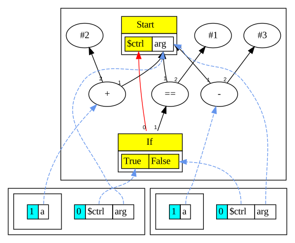
* Note the two `ScopeNode`s in the graph.
* One has its `$ctrl` pointing to the `True` projection, while the other has `$ctrl` pointing to `False` projection.
* Note that `a` is bound to the `Sub` node in the `False` branch, whereas `a` is bound to the `Add` node in the `True` branch.
* Thus `a` needs a `Phi` node.
### After merging
Below is the graph after we created a `Region` node and merged the two definitions of `a` in a `Phi` node.
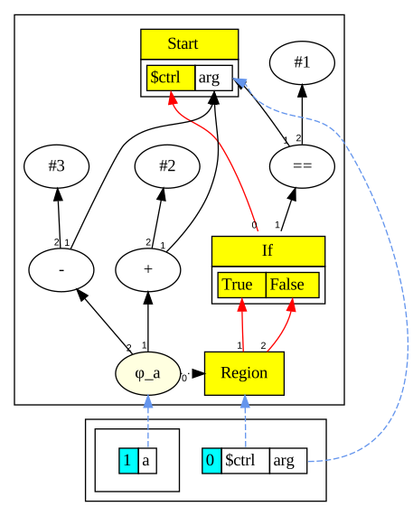
* Observe that the duplicate `ScopeNode` has been discarded.
* `a` is now bound to the `Phi` node.
* The `Phi` node's inputs are the `Region` node and the `Add` node from the `True` branch, and `Sub` node from the `False` branch.
### Finally
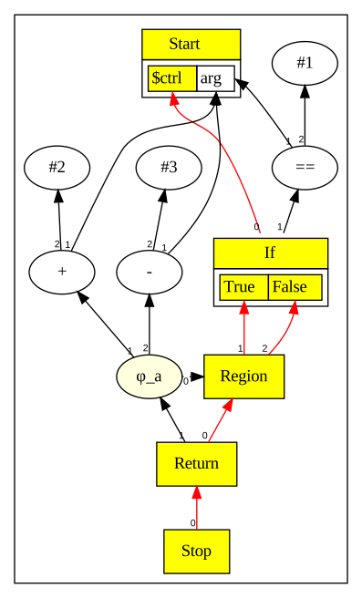
Here is the graph after the `return` statement.
## References
[1]
Click, C. (1995).
Combining Analyses, Combining Optimizations, 132.
[2]
Click, C. (1995).
Combining Analyses, Combining Optimizations, 102-103.
[3]
Click, C. (1995).
Combining Analyses, Combining Optimizations, 129.
[4]
Click, C. (1995).
Combining Analyses, Combining Optimizations, 86.